Every Frame Is a Memory Read: A Systems View of Speech Model Inference on Apple Silicon

Everything I tried, on one chart. Left: the accepted ladder, drift-corrected — 3.19× → 4.98× real-time (1.56×); the hatched fourth bar is a 4-bit code predictor that failed the quality gate, and whose RTF overstates it (§6). Right: each lever against its own parent; hatched bars bought nothing or failed the gate, † marks runs the harness flagged for contention. Measured.

The last post ended with a number I didn’t like: almost all of a GRPO step is spent in Phase A, sampling rollouts. The ASR pass that everyone assumes is the bottleneck was about 3% of step time. Making the policy learn faster turned out to mostly mean making the policy speak faster.

This post is about that, and it ended up being as much about measuring as about optimising. The model is the same one the series has been building on — Qwen3-TTS with my Hindi adapters, on an M5 Pro, in MLX. The story has three parts: this is the baseline, this is what I changed, this is where it got me. Most of the techniques come from the CUDA serving world. Some transferred. Several didn’t, and the reasons they didn’t are the most useful part of the post.

The short version:

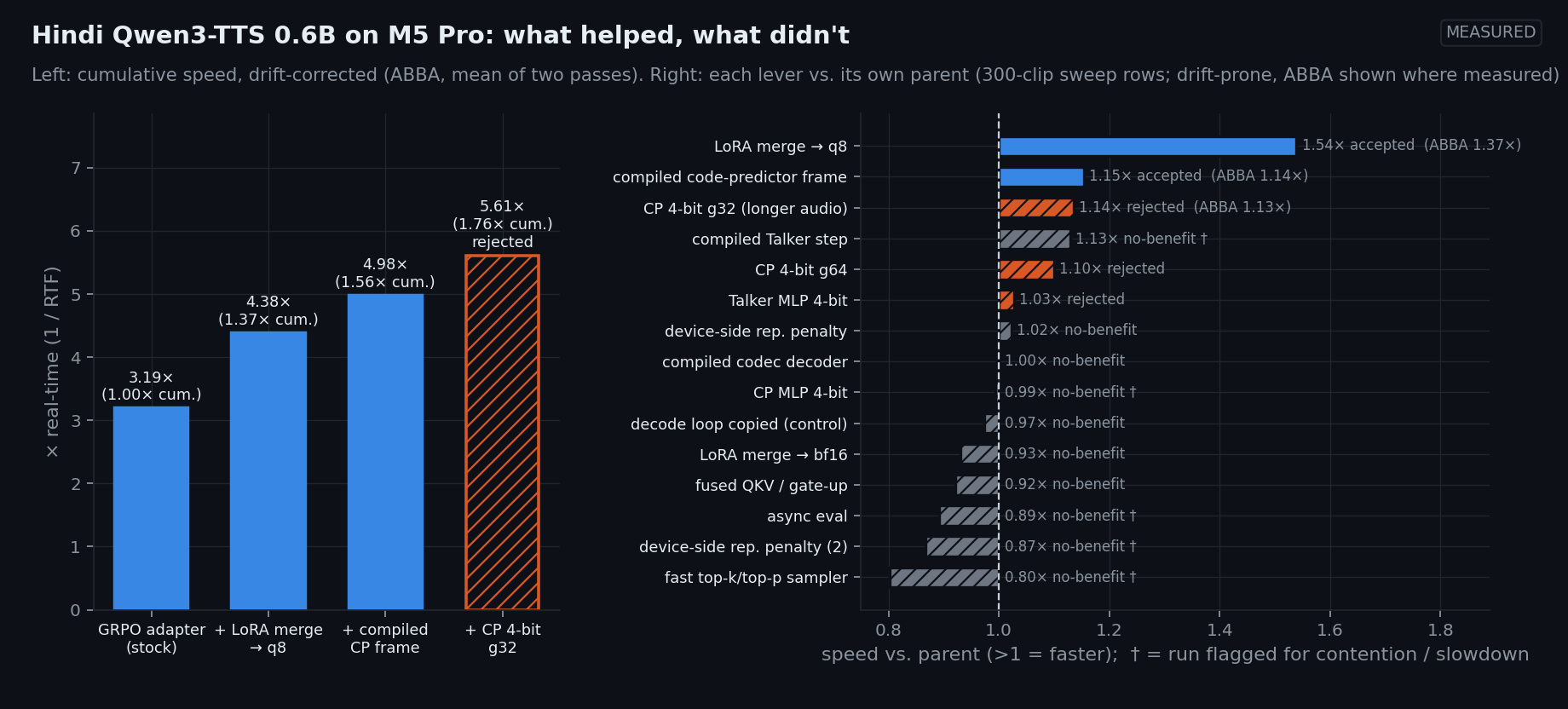
• Two changes made single-stream generation 1.56× faster (3.19× → 4.98× real-time, drift-corrected): merging the LoRA adapter into the 8-bit weights, and compiling the code predictor’s fifteen passes into one graph. On 300 new held-out sentences they showed no statistically detectable degradation in CER or DNSMOS, within stated margins. That is automatic metrics only; nobody has blind-rated it yet.
• A 4-bit code predictor looked like another 1.13× and was rejected. On new sentences it lowered DNSMOS; it says the same text in ~7% more audio, so most of its “speedup” was a longer output; and given identical inputs it changes about a third of the code predictor’s token draws.
• Ten changes did nothing and three were rejected. Every one of them is in the ledger with the reason.
• The largest 8-bit matvecs, measured in isolation, move their weights at about the M5 Pro’s DRAM spec. The whole frame is still ~1.5× off the first-order roofline; what’s left is mostly structure — or a model change.
• The numbers misled me seven times — single-run noise, macOS background scans, a dictation app, thermal drift, a DNSMOS “regression” that was seed luck, my own per-clip statistics, and a speed metric that rewards talking longer. The method section is the story of how the harness learned to catch each one.

Results at a glance

Configuration	Speed	Quality vs. its parent (per sentence, 95% CI)	Evidence	Status
GRPO adapter, stock mlx-audio	3.19× real-time	—	A-B-B-A, 2 × 100 sentences	baseline
+ LoRA merged into the q8 weights	4.38× (1.37×)	ΔCER −0.002 [−0.012, +0.008]; ΔDNSMOS −0.014 [−0.038, +0.005]¹	A-B-B-A speed; quality on 300 new sentences	accepted
+ compiled code-predictor frame	4.98× (1.56× cumulative)	bit-identical to the row above	A-B-B-A; 300/300 clips bit-identical	accepted
+ 4-bit code predictor (group 32)	1.13× by RTF, 1.02–1.07× wall-clock	ΔDNSMOS −0.040 [−0.063, −0.015]; audio 7% longer	300 new sentences; teacher-forced check	rejected
Batched GRPO rollouts (G = 16)	2.10× throughput vs. G = 1	descriptive only	20 sentences × 2 seeds, one run	preliminary

¹ Measured with the compile step on top, which is bit-identical, so the change is the merge's. Margins: CER +0.02, DNSMOS −0.05 (§2). All quality results are automatic metrics.

Prerequisites: This is the fourth post in the speech series — representation (From Spectrograms to Speech Codecs), generation (Inside the Speech LM), refinement (GRPO Post-Training for TTS), and now inference. The roofline method comes from Running Conversational AI Locally: decode is a memory read, so bytes per step divided by bandwidth predicts the step time. If “the Talker predicts codebook 0 and a smaller module fills the other fifteen” is familiar, you’re ready.

---

Contents

1. Why inference speed matters — and four things I got wrong
2. Baseline and method
3. Predict first: the roofline
4. Where the time goes: profiler and GPU telemetry
5. The ladder: what worked, what didn’t
6. Seven times the numbers lied
7. Results: baseline to final
8. Beyond one stream: batching, and what changes at scale
9. What’s still open

Appendix: reproduce it

---

1. Why inference speed matters

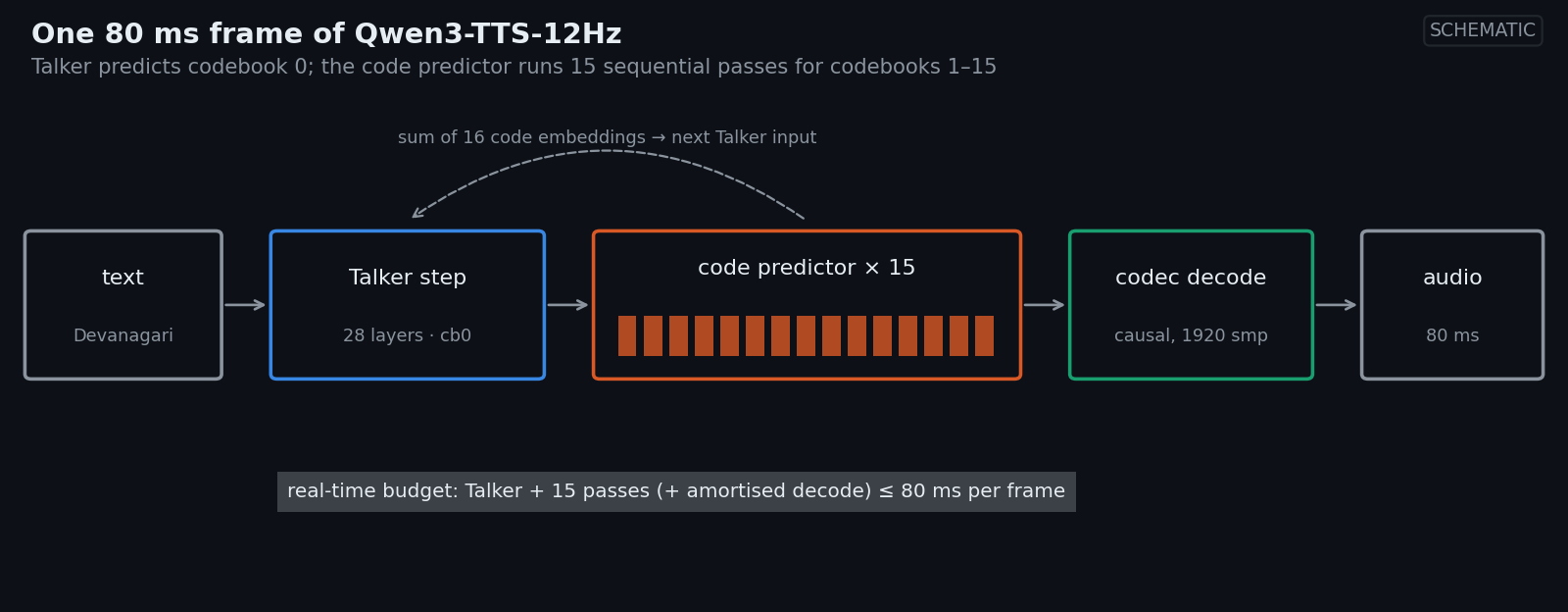
A one-paragraph refresher on the model, because everything below depends on it. Qwen3-TTS generates speech as frames of sixteen codec tokens, one frame per 80 ms of audio. A 28-layer transformer, the Talker, predicts the first token of each frame; a small 5-layer code predictor then fills in the other fifteen, one at a time; a causal codec decoder turns frames into waveform.

One 80 ms frame. The Talker predicts codebook 0; the code predictor runs fifteen sequential passes for codebooks 1–15; the sum of all sixteen code embeddings becomes the next Talker input. Decode runs per chunk, so its cost is amortised across frames. Schematic.

Two reasons, one for each half of the series.

Training. GRPO samples a group of G rollouts per prompt, decodes them to audio, transcribes them, scores them, and takes one gradient step. Sampling is most of the step, so every millisecond off a decode frame comes off training, G times per prompt.

Deployment. Qwen3-TTS’s streaming tokenizer emits a frame every 80 ms (12.5 Hz). If producing a frame takes longer than 80 ms, playback starves. That number is the budget for everything in this post.

Four things I got wrong earlier

Before measuring anything I read the code path mlx-audio actually runs, and it disagrees with my own earlier posts in four places.

1. The decoder has no DiT and no denoising loop. In the May post I wrote that Qwen3-TTS decodes through a flow-matching DiT and then BigVGAN. That’s true of one of its two tokenizers. The paper describes a 25 Hz single-codebook tokenizer that reconstructs waveforms with a block-wise flow-matching DiT and a modified BigVGAN, and a separate 12 Hz multi-codebook tokenizer that needs only “a lightweight causal ConvNet”. The released models I use, and that mlx-audio loads, are the 12 Hz ones. In mlx-audio the decoder is RVQ dequantization, an 8-layer transformer with a 72-frame sliding window, then causal transposed-conv upsampling with SnakeBeta activations: 8·5·4·3 × 2·2 = 1920 samples per frame, and 24,000 / 1920 = 12.5 Hz. “12Hz” is a rounded name. vLLM-Omni’s write-up calls it a lightweight non-DiT decoder, and that’s correct.

2. The MTP module is not “one shot”. Both earlier posts say the multi-token-prediction module fills the 15 residual codebooks in one parallel step. In mlx-audio the module (talker.code_predictor, a 5-layer transformer, hidden size 1024) runs 15 sequential passes per frame, one per residual codebook, each sampling a token that feeds the next pass. The paper’s “single-frame instant generation” is about latency at frame granularity, not a single forward pass. This turns out to be the most consequential correction in the post: §3 shows it’s where most of the bytes go, and §4 shows it’s where most of the time goes.

3. The speed estimate. The May post said a 1.7B step takes “roughly 8–12 ms” on an M5 Pro, giving “~7–10× real-time”. That was an estimate, for a model size I’m not using, and it ignored the code predictor. The measured baseline for the model I actually deploy is 3.19× real-time; the best accepted configuration is 4.98× (§7).

4. “LoRA fuses into the base at no cost.” The appendix of the May post says this. My adapters sit on an 8-bit base, and in mlx-audio-train only the full-precision LoRALinear has a fuse() method; the QLoRALinear wrapper used on a quantized base has none. So the deployed adapter has always run unmerged: two extra skinny matmuls, a scale and an add on every one of 231 wrapped projections — the Talker’s 28 layers and, through the talker scope, the code predictor’s 5 layers, which run fifteen times a frame. §5.1 measures what that cost: it was the single biggest lever in the post.

Two smaller findings came out of reading the training code, and they matter for anyone who reuses it:

• LoRA dropout is on at inference. MLX’s loader puts the model in eval mode, but apply_lora then inserts 231 fresh Dropout(0.05) layers, which default to training mode, and nothing switches them off — not in grpo_heldout_eval.py, not in the demo, not in GRPO rollouts or the KL reference forward. Every benchmark here calls model.eval(). The GRPO post’s held-out CER was measured with dropout still on, and its “KL is exactly 0 at step 0” invariant can’t strictly hold when the policy and reference forwards draw different dropout masks.
• GRPO doesn’t sample the way deployment does. The GRPO sampler uses no repetition penalty; mlx-audio’s generate() uses 1.05. Small, but the GRPO post’s whole lesson was to match the deployment path.

One scoping note: the Hindi adapters from the last two posts are trained on Qwen3-TTS-12Hz-0.6B-Base-8bit, so this post is about the 0.6B model.

---

2. Baseline and method

The baseline

Framework	MLX 0.31.2, mlx-audio 0.4.4 (stock generate())
Code	every lever is one change on top of that baseline, in mlx-audio-train/bench
Model	mlx-community/Qwen3-TTS-12Hz-0.6B-Base-8bit
Variants	stock (no adapter); Hindi SFT and Hindi GRPO LoRA adapters (rank 8, α 16) on the 8-bit base, unmerged. The ladder is measured on the GRPO adapter — the one I deploy.
Device	M5 Pro, 64 GB
Sampling	temperature 0.9, top-p 0.95, top-k 50, repetition penalty 1.05, ≤ 240 frames
Prompts	100 held-out Hindi sentences from IndicTTS-Hindi (median 76 characters, ~10 s of speech; 58 female / 42 male source speakers) × 3 seeds = 300 clips per configuration

The adapters were trained on IndicVoices-R, so these sentences are unseen. It also means CER here is not comparable to the GRPO post’s numbers, which came from an IndicVoices-R held-out set. The original held-out file from that post no longer existed on my disk; scripts/make_prompt_set.py --n 100 --seed 0 rebuilds this one exactly.

The harness

The protocol started from VoiceHub’s TTS optimization benchmarks, which record every candidate, including rejections, in a machine-readable ledger and time with a fixed seed, a fresh process, warm-ups, repeated runs and a 10-second minimum. Mine grew from there — several of the rules below exist because a measurement fooled me first (§6):

• One configuration per fresh process, one warm-up generation discarded, then an uninstrumented speed pass over all 300 clips (~40 minutes of audio).
• One change at a time. Every ledger row names its parent, so each lever is judged against exactly the configuration it modifies.
• Force evaluation before reading the clock. MLX is lazy: nothing runs until something forces it, and a timer around unevaluated code measures graph construction. Every timed region ends with mx.eval.
• Two kinds of run. Forcing evaluation at component boundaries (to split the Talker from the code predictor from the decoder) adds syncs that change what’s being measured, so the component breakdown comes from a separate, instrumented pass and is never used for speed claims.
• Bit-exactness check. Each clip’s waveform is hashed; a lever that should not change the output either reproduces the parent’s audio exactly or fails.
• Contention and telemetry. Every run records any other process above 40% CPU and, from the moment I learned it mattered, GPU utilisation, GPU clock, power, temperatures and swap via macmon during the timed pass (§4).
• Drift correction for headline numbers. The final ladder is re-measured back-to-back in A-B-B-A order (§6, §7).

Metrics

Metric	Definition
RTF	wall time ÷ audio duration (lower is better); × real-time = 1 / RTF
TTFP	time from call to the first streamed audio chunk (default 2 s streaming interval)
Talker ms/step	one Talker forward (instrumented pass)
Code predictor ms/frame	all fifteen passes for one frame, including their sampling once compiled (instrumented pass)
Codec ms	decoder ms per second of generated audio
CER (capped)	per-clip Whisper-large-v3-turbo CER capped at 1.0, as in the GRPO sweep
DNSMOS OVRL	reference-free quality; English-trained, so a relative indicator on Hindi

The quality gate

A lever is accepted only if it is faster and passes the gate:

• Speed: faster by at least 3% and by more than the measured run-to-run spread.
• Quality: output bit-identical to the parent — then quality is unchanged by construction — or non-inferior on the automatic metrics.

“Non-inferior” needs defining, because the obvious version — “not significantly worse” — is too weak: a small or noisy sample passes it by default. The gate works like this:

• The unit is the sentence, not the clip. 300 clips are 100 sentences × 3 seeds; clips of the same sentence aren’t independent, and once outputs diverge seed-matched clips aren’t true pairs. Each configuration’s CER and DNSMOS are averaged over seeds per sentence, and the difference to the parent is taken per sentence.
• Each difference gets a 95% confidence interval, bootstrapped over sentences.
• Non-inferiority margins: capped CER may rise by at most +0.02 (absolute), DNSMOS OVRL may drop by at most 0.05. A lever passes only if the worst end of the interval is inside the margin.
• Same text, same length. Per-sentence audio length must stay within ±3% (both ends of its interval), and speed is judged on the smaller of the RTF and wall-clock speedups. This rule came last, from §6’s seventh lie.

Two honest caveats. The DNSMOS threshold was fixed early; the CER margin, and the switch to sentence-level intervals, came after the ladder had run, when a review pointed out that my original per-clip tests treated 300 clips as 300 independent observations. Every quality claim below was re-analysed under the stricter gate, and two verdicts changed wording (§6). Second, all of this is automatic metrics only: Whisper CER and an English-trained DNSMOS. Passing the gate means no statistically detectable degradation on those metrics, not “sounds the same” — that needs blind listening by native Hindi speakers, which hasn’t happened yet (§9).

Anything slower or not significantly faster is no-benefit; anything that fails quality is rejected. All three stay in the ledger.

---

3. Predict first: the roofline

The March post’s method: during decode the weights are read once per step and there’s very little arithmetic per byte, so

time per step ≈ bytes read per step / (peak bandwidth × utilization)

On the M1 I measured 65–69% of peak bandwidth during LLM decode. I used that range for the M5 Pro (307 GB/s) before measuring anything.

Counting the bytes

From the published 0.6B config:

• Talker: 28 layers, hidden 1024, MLP 3072, 16 query heads and 8 KV heads of dimension 128 — 15.7M parameters per layer, plus a 3072-way codec head: 443.5M parameters read per step.
• Code predictor: 5 layers of the same width, plus the one 2048-way head used at that pass: 80.7M parameters per pass, × 15 passes.
• KV cache: 112 KB per token; ~31 MB at a typical context, small next to the weights.

At q8 — MLX affine quantization, group 64, about 8.5 bits per weight — a frame reads 0.50 GB for the Talker and 1.29 GB for the code predictor. The fifteen small passes read 2.6× more than the Talker does.

One decode frame is a memory read: the Talker's weights once, the code predictor's fifteen times. At q8 that's ~1.79 GB per frame. Predicted, not measured.

The predictions I committed to

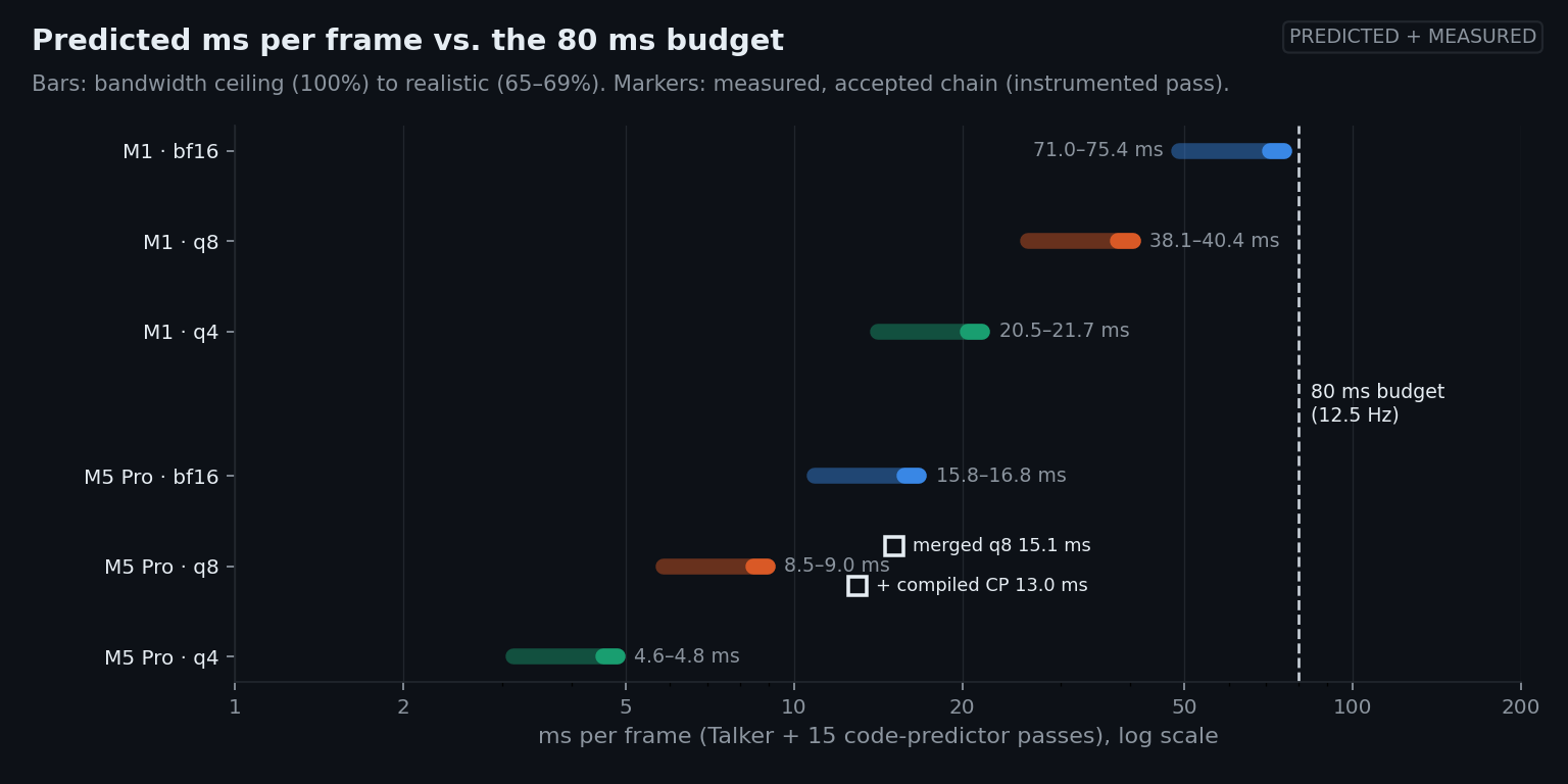
Device	Precision	GB / frame	ms / frame @ 100%	ms / frame @ 65–69%
M5 Pro (307 GB/s)	bf16	3.34	10.9	15.8–16.8
M5 Pro	q8	1.79	5.8	8.5–9.0
M5 Pro	q4	0.97	3.1	4.6–4.8

1. The adapters’ base (q8) should spend 8.5–9 ms per frame in the Talker and code predictor, ~9× real-time before decode.
2. Precision scales the frame time almost linearly — q8 → q4 another ≈ 1.9×.
3. The code predictor will miss its roofline by more than the Talker. One pass reads ~86 MB; at that size the fixed cost of launching a pass’s kernels is no longer small next to the memory time, and there are fifteen passes per frame.

How they fared (§7 has the full comparison): prediction 3 was right, and it drove the whole optimisation. Prediction 2 was badly wrong — 4-bit bought 1.15× on the code predictor, not 1.9× — and the kernel microbenchmark in §4 explains why. Prediction 1 was wrong at baseline by 2–3× and ended up within ~1.4× after the two accepted levers.

The roofline, per device and precision, with the two accepted M5 Pro configurations overlaid: merged q8 at 15.1 ms and with the compiled code predictor at 13.0 ms of Talker + code predictor per frame (instrumented pass). The M1 rows are predictions only. Predicted + measured.

---

4. Where the time goes

The baseline breakdown

The first measurement of the GRPO adapter on stock mlx-audio, per frame, instrumented pass (300 clips):

Component	Measured	Predicted (q8)	Measured ÷ predicted
Talker step	5.83 ms	2.4–2.5 ms	~2.4×
Code predictor, 15 passes	18.36 ms	6.1–6.5 ms	~2.9×
Codec decode	22.6 ms per second of audio (~1.8 ms per frame)	—	—

Both components are far off the roofline, and the code predictor is further off — prediction 3, in numbers.

A layer-by-layer profiler, and its tax

To go deeper I wrote a profiler (scripts/bench_profile.py) that brackets modules with forced evaluation. The first thing it measured was itself: each bracket costs ~130 µs of sync on the M5 Pro — more than most individual layers take. Bracketing every projection inside the code predictor added ~1,700 syncs per frame and turned a 25 ms frame into 300 ms of mostly profiler. So it profiles one level at a time, in a fresh process each, and subtracts the calibrated sync cost. At level 1 (components), the corrected total came to 25.3 ms against 24.8 ms measured uninstrumented — close enough to trust:

Component (per frame, smoke set)	GRPO adapter (unmerged LoRA)	Stock, no adapter
Code predictor (15 passes × 5 layers + head)	15.0 ms (59%)	9.4 ms (55%)
Talker (28 layers + codec head)	5.6 ms (22%)	3.3 ms (19%)
Codec decoder (amortised)	1.9 ms	1.9 ms
Code-predictor sampling (15 per frame)	1.6 ms	1.5 ms
Python / glue / per-frame sync	1.0 ms	1.0 ms
Talker sampling + embedding lookups	~0.2 ms	~0.2 ms
Total	25.3 ms	17.2 ms

Two conclusions fell straight out of this table:

1. The unmerged LoRA costs 31% of the frame (25.3 vs 17.2 ms) — 5.6 ms in the code predictor and 2.3 ms in the Talker. The bytes are negligible (~24 MB); the ~2,900 extra kernel launches per frame are not.
2. The code predictor is over half the frame either way. Inside a layer, attention costs ~0.16 ms and the MLP ~0.10 ms per call, identical in the Talker and the code predictor (same shapes) — but the code predictor makes 75 layer calls per frame against the Talker’s 28.

What the GPU was doing

Wall-clock time says how long; it doesn’t say whether the GPU was busy, how fast it was clocked, or how hot it was. From the second half of the experiments on, every timed pass ran macmon (sudo-free Apple Silicon telemetry, 500 ms samples) alongside. Over the timed speed passes of the configurations built on the merged, compiled model:

Configuration (300 clips)	GPU busy	GPU clock (mean / max)	GPU power	System power	GPU temp (max)
+ compiled Talker step	89%	1497 / 1620 MHz	8.6 W	41.6 W	75.4 °C
+ compiled decoder	88%	1521 / 1616 MHz	9.0 W	41.6 W	71.6 °C
+ code predictor 4-bit g64	89%	1532 / 1617 MHz	9.1 W	39.9 W	71.3 °C
+ code predictor 4-bit g32	90%	1538 / 1617 MHz	9.6 W	44.5 W	72.5 °C
+ fused projections	86%	1470 / 1613 MHz	8.5 W	44.7 W	74.3 °C
+ fast sampler †	82%	1485 / 1614 MHz	7.1 W	37.2 W	70.8 °C
+ code predictor MLP 4-bit †	86%	1506 / 1616 MHz	8.6 W	40.4 W	70.2 °C
+ Talker MLP 4-bit	89%	1529 / 1605 MHz	9.0 W	40.0 W	72.8 °C

† runs the harness flagged for contention or a machine-wide slowdown (§6).

Three things this table says:

• “Busy” is not “efficient”. At batch 1 the GPU reports 86–90% busy, yet most of its kernels are small matrix-vector products. The utilisation counter measures the fraction of time the GPU has work, not how much of its bandwidth or compute that work uses. A frame of many hundreds of tiny kernels (540 matmuls in the code predictor alone) keeps it busy and still leaves throughput on the table — which is exactly the headroom batching uses (§8).
• The GPU runs ~5–9% below its peak clock (1.47–1.54 GHz mean against 1.60–1.62 GHz max), at only 7–10 W. Bursty small-kernel decode doesn’t hold the clock at maximum. On a laptop there’s no knob for this; it’s part of the environment the levers live in.
• Temperatures climbed into the low 70s during long runs. Over hours of back-to-back runs the whole machine drifted ~12–15% slower — on every component at once, including the decoder no lever touched. That’s what forced the A-B-B-A re-measurement in §7.

A rough energy figure falls out too: at ~5× real-time and ~9 W of GPU power, one second of Hindi speech costs about 1.8 J of GPU energy (~8 J for the whole system).

How close to the hardware are the matmuls?

The last measurement explains why prediction 2 failed, and where the floor is. scripts/bench_kernels.py, on an idle machine:

Fixed cost per GPU kernel: ~1.9 µs — the slope of N dependent tiny matmuls, compiled or not.

8-bit matvec efficiency depends on size (input 1024, timed as a dependent chain):

Output size	q8 time	q8 % of peak bandwidth	q4 % of peak
1024 (K, V projections)	7.8 µs	47%	25%
2048 (Q projection, code-predictor heads)	9.7 µs	75%	41%
3072 (MLP gate/up)	11.0 µs	99%	55%
6144 and up	20.7 µs+	100–130%	86–124%

Three different numbers are easy to blur here, so to be precise about what this table is:

• 307 GB/s is the M5 Pro’s nominal DRAM bandwidth — a spec, not something I measured.
• The percentages are effective throughput: weight bytes divided by time for one isolated matvec, repeated in a dependent chain. Nothing guarantees those bytes came from DRAM. Above 100% they clearly didn’t all — the small weight matrices are partly served from the on-chip cache — and at 99% I can’t separate DRAM traffic from cache hits either. I didn’t measure DRAM traffic directly; macmon doesn’t expose it.
• End-to-end frame time is a third thing. It includes the non-matmul work, the smaller and less efficient matvecs, sampling and glue (below), and it sits at ~1.5× the roofline prediction (§7).

So “99%” means: an 8-bit matvec of the MLP’s shape, in isolation, moves its weights as fast as the DRAM spec allows. It does not mean the decode loop runs at 99% of DRAM bandwidth, and the roofline itself is a first-order model — bytes over bandwidth, ignoring caches, launch latency and overlap.

At the code predictor’s sizes, a 4-bit matvec is barely faster than an 8-bit one (10.5 vs 11.0 µs at 3072): halving the bytes doesn’t help when a fixed per-kernel latency dominates. That is why 4-bit bought 1.13–1.15× instead of the predicted 1.9×.

One compiled code-predictor frame, decomposed: its 540 matmuls alone take 5.90 ms; the real compiled frame takes 8.42 ms. The remaining 2.52 ms (30%) is everything that isn’t a matmul — norms, RoPE, attention over ≤ 17 cached keys, sampling, glue. That 30% is the most a fused custom kernel could ever recover (§9).

What the CUDA work suggests

This is not a speed comparison — a data-centre GPU at concurrency 64 and a laptop at batch 1 aren’t measuring the same thing. The useful question is whether the diagnosis transfers. vLLM-Omni’s TTS team found the same shape of problem at serving scale. At concurrency 64 on two H20s, average GPU utilization for the Talker stage and the Code2Wav stage was about 14% and 6%; in their words, “the GPU was often waiting on Python scheduling”, small allocations and kernel-launch overhead. On a single laptop stream the GPU is busy — 86–90% — but the work is fragmented into kernels too small to use it well. Same disease, different symptom.

---

5. The ladder

Each lever: where the idea came from, what the baseline did, the change, and the measured result on 300 clips with its decision. The waterfall at the top of the post is the summary; the ledger has every row.

Before writing any lever I looked at what others had done to make Qwen3-TTS and similar models fast. The table is about which ideas transfer to MLX on Apple Silicon, not about whose numbers are bigger: the platforms, batch sizes and models differ, and none of their speedups is comparable to mine.

Source	Platform	What they did	What happened here
faster-qwen3-tts	CUDA	Static KV cache + CUDA graphs over the Talker and the whole 15-step code predictor; vectorised repetition penalty	The code-predictor capture transferred (§5.2). The Talker capture and the device-side penalty didn’t — MLX’s loop wasn’t sync-bound the way PyTorch’s was.
faster-qwen3-tts, what didn’t help	CUDA	Fused RMSNorm/SiLU kernels: 8.4×/2.2× faster alone, 1.25× end to end; “Attention is not the bottleneck.”	Same lesson: launch count, not elementwise math.
qwen3-tts-triton	CUDA	Triton RMSNorm, SwiGLU, M-RoPE, norm+residual: 1.1× alone, 5× with CUDA graphs	Same lesson again.
Single-kernel Qwen3-TTS	RTX 5090	A persistent “megakernel” running the Talker and code predictor	Concept only: Metal has no public device-wide barrier (§9).
Soniqo Swift/MLX port	Apple Silicon	Runs the 15-group code-predictor loop as one compiled graph; “int4 was decommissioned for TTS quality”	Independent support for both the accepted compile lever and the 4-bit results.
ML Drift (Google)	Metal / OpenCL / WebGPU	Weight-layout fusion (QKV), mixed 8/4/4 quantization	Fused projections: no benefit (§5.6). Selective 4-bit: rejected (§5.8).
MLX decode proposals	MLX	Fused sampler, skipping full-vocabulary log-softmax, FP8 KV cache	Fast sampler: no benefit (§5.6). FP8 KV: not tried — the KV cache is ~6% of the bytes.
FluidInference (mobius)	CoreML / Neural Engine	A Qwen3-TTS CoreML port; PocketTTS on the ANE	Their Qwen3-TTS port runs ~6–10× slower than real time: 16 CoreML calls per frame because the code-predictor loop wouldn’t trace — “per-prediction CoreML overhead, not the actual neural network compute”. Their PocketTTS split of work across ANE and GPU measured no gain (−0.9%). Their selective-int8 recipe inspired §5.8.
vLLM-Omni	CUDA serving	Async/sync removal, whole-forward compile, staged Talker/Code2Wav	Sync removal: no benefit here (§5.5). Staging: §8.

5.1 Merge the LoRA into the 8-bit weights — accepted, 1.37×

Baseline: 231 unmerged QLoRALinear projections, each adding two skinny matmuls, a scale and an add — ~2,900 extra kernels per frame.

Change: dequantize each wrapped base weight, add scale · B·A in float32, requantize with the base’s own group size and bits (bench/lora_merge.py). The merged layer’s output differs from the unmerged one by 0.76% (median relative error) — the requantization rounding.

Result: 1.54× in the sweep (2.88× → 4.43× real-time); 1.37× in the drift-corrected A-B-B-A re-measurement, which is the number I quote. Talker 5.83 → 3.31 ms, code predictor 18.36 → 11.80 ms, time to first packet 756 → 419 ms, peak memory 7.6 → 6.7 GB.

Quality, per sentence against the unmerged parent: on the original 100 sentences, ΔCER +0.007 [95% CI −0.005, +0.020] and ΔDNSMOS −0.011 [−0.050, +0.025] — both upper/lower bounds sitting right on the margins, so that sample couldn’t establish non-inferiority either way. I re-ran the merge (with the bit-identical compile on top) against the baseline on 300 new IndicTTS sentences, one seed each: ΔCER −0.002 [−0.012, +0.008], ΔDNSMOS −0.014 [−0.038, +0.005]. Both intervals sit inside the margins — no statistically detectable degradation on the automatic metrics.

The adapted model now runs at stock speed (4.43× vs 4.33× for the base model with no adapter). Merging into bf16 instead was no-benefit (0.93×): it removes the LoRA kernels but doubles the bytes of the merged layers. That pair of rows is the bandwidth-vs-launch trade-off in its simplest form.

5.2 Compile the code-predictor frame — accepted, 1.14×, bit-identical

Borrowed from: CUDA graphs, as faster-qwen3-tts captures the whole 15-step code predictor, and Soniqo’s compiled 15-group loop. vLLM-Omni compiled VoxCPM2’s whole forward and cut its kernel-launch count by 71%.

Change: the whole frame — fifteen passes of five layers, the heads, the sampling, and the sum of codebook embeddings — becomes one mx.compile‘d function (bench/fast_generate.py). Inside the trace the stock modules are reused, with the KV cache replaced by a pure concatenating cache that returns the same keys and values; the random state is a compile input and output, so sampling consumes the same keys as stock.

Result: bit-identical to its parent on all 300 clips, and 1.14× faster (1.15× in the sweep). The code predictor drops from 11.8 to 9.2 ms per frame — half of its original 18.4 — and the separate sampling cost disappears into the graph.

FluidInference couldn’t do this in CoreML: tracing froze SDPA’s causal mask, so they ended up with sixteen model calls per frame. MLX’s tracer handled the same loop without a single change to the model code.

5.3 Compile the Talker step — no-benefit

Change: the Talker decode step on fixed-shape K/V slot buffers (capacity rounded to 64), written with slice_update and masked, one trace per utterance. Bit-identical.

Result: 0.98×. The sweep row first came out “accepted 1.13×” — against a parent that a dictation app had slowed by 13% (§6). Against the clean configuration it’s 0.98×, and the Talker’s own step time didn’t move (3.76 vs 3.82 ms). The Talker was never launch-bound: 28 layer calls per frame, ~1.5× its roofline. Fixed-capacity buffers add their own cost — every step attends over ~400 slots and rewrites 56 slot buffers.

5.4 Compile the codec decoder — no-benefit

Change: right-pad codes to a 16-frame bucket, decode with one compiled decoder per bucket, trim. Valid only because every decoder stage is causal; the padded, compiled output was bit-identical to stock at every tested length.

Result: 1.00×. The decoder is heavy 24 kHz convolution — compute, not launches — and at ~1.8 ms per frame it was never the problem. (fast-dacvae got 5× on a different codec on an H100 with CUDA graphs; this decoder had no such overhead to remove.)

5.5 Overlap the per-frame sync — no-benefit

Borrowed from: vLLM-Omni removing .item() syncs from VoxCPM2’s Euler loop.

Baseline: mlx-audio already has a single sync per frame (the code even says so: “Single sync point”). But the repetition penalty is built from a Python list of generated tokens, so sampling frame t+1 needs frame t’s token on the host — there is nothing to overlap until the penalty moves to the device.

Changes: first the penalty from a fixed-shape device-side mask (bit-identical, 1.02×), then mx.async_eval with the EOS check one frame late (bit-identical, no gain — 1.005× on a clean smoke run; the 300-clip row ran during contention). The GPU was never waiting on the CPU between frames.

The CUDA-world picture of a sync-bound decode loop, and the fix. On MLX the measured gap wasn't there: async evaluation was bit-identical and bought nothing. Schematic.

5.6 Fewer launches, two ways — no-benefit

Once the code predictor was compiled, I tried the two remaining launch-count ideas from the survey:

• Fused QKV and gate/up projections (ML Drift’s layout fusion): q/k/v concatenated into one quantized matmul and gate/up into another — 7 matmul launches per layer become 4. Bit-identical (max difference 0.0), 0.92×. In isolation a bigger matvec is more efficient (§4); inside the compiled frame the fused version wasn’t faster.
• A cheaper sampler (MLX decode proposals): top-p over the 50 top-k survivors instead of sorting all 2,048 entries, scattered back into a full-vocabulary draw so the random numbers line up. 275 of 300 clips bit-identical (the rest differ by rounding at the top-p threshold), no quality change, no speed gain. That row ran during a machine-wide slowdown (§6); the clean smoke run was 0.98×.

Both confirm the same thing: after compilation, dispatch overhead is no longer where the time is.

5.7 Smaller ideas, not built

• Preallocated code-predictor KV buffers (Fish Speech’s fast-AR path in vLLM-Omni): moot once the frame is compiled — inside the trace the cache is a pure concatenation.
• Sliding-window decode instead of re-decoding the prefix (VoxCPM2’s O(N²) → O(N) fix): already in the baseline. mlx-audio’s streaming path decodes incrementally, and my GRPO trainer decodes each rollout once.
• Caching reference-audio features for voice cloning: not on this path — the Hindi adapter doesn’t use a reference clip.

5.8 Quantization behind the gate — four variants, one survivor

Borrowed from: VoiceHub’s ledger, whose F5-TTS BF16 entry (2.86× faster, WER 0.485 → 1.455) was rejected; FluidInference’s selective int8 recipe and ML Drift’s 8/4/4 split.

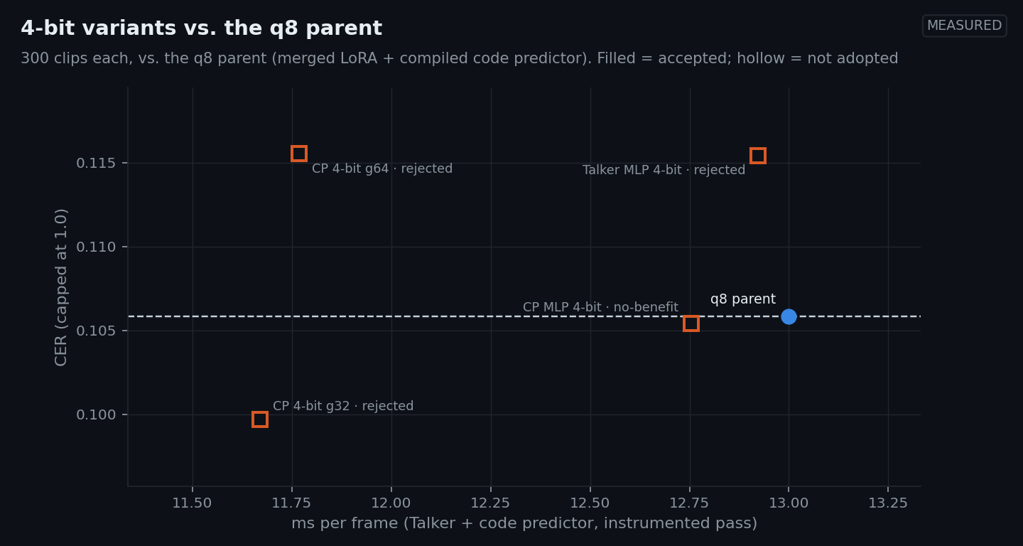
All four start from the accepted configuration (merged q8 + compiled code predictor) and change only precision:

Quality is the per-sentence change against the q8 parent on the original 100 sentences (seeds averaged), with a 95% CI; margins are +0.02 CER and −0.05 DNSMOS. The group-32 row was then re-tested on 300 new sentences — below the table.

Variant	Speed vs. parent	Per-layer error	ΔCER [95% CI]	ΔDNSMOS [95% CI]	Decision
Code predictor 4-bit, group 64	1.10×	9.3%	+0.010 [−0.005, +0.024]	−0.005 [−0.044, +0.040]	rejected — CER bound outside margin
Code predictor 4-bit, group 32	1.13× (A-B-B-A); 1.07× wall-clock	8.3%	−0.006 [−0.020, +0.006]	+0.025 [−0.015, +0.068]	passed here; rejected on new sentences
Code predictor MLP only, 4-bit (attention + heads q8)	0.99× †	9.3%	−0.000 [−0.015, +0.013]	−0.033 [−0.077, +0.013]	no-benefit (DNSMOS bound also outside margin)
Talker MLP only, 4-bit (attention + head q8)	1.03×	9.4%	+0.010 [−0.004, +0.023]	−0.013 [−0.070, +0.042]	rejected — both bounds outside margin

Four 4-bit variants against their q8 parent, 300 clips (100 sentences × 3 seeds) each, on CER alone. The group-32 code predictor looked clean here; it failed on DNSMOS and output length when re-tested on new sentences. Measured.

Three readings of the first round:

• Group size looked like it mattered more than which layers. Group 64’s CER interval reaches +0.024, past the margin; group 32 (finer scales, ~0.5 bit per weight more) stayed inside it on both metrics.
• “Selective” didn’t rescue 4-bit in the Talker. Keeping attention and the head at q8, as FluidInference and ML Drift do, still left the Talker MLP variant outside both margins, and its CER shift is consistent across sentences (sentence-level Wilcoxon p ≈ 0.001) even though the mean is small. Soniqo reached the same place independently.
• The speed gain is small — 1.10–1.13× for halving the bytes — for the reason §4 measured: at these matrix sizes 4-bit matvecs are latency-bound.

Why group 32 didn’t survive

Group 32 was the one variant that passed, so I tried to break it before believing it, three ways.

New sentences. On 300 IndicTTS sentences the ladder had never seen, one seed each, against the merged-and-compiled q8 parent: ΔCER +0.000 [−0.009, +0.010] — fine — but ΔDNSMOS −0.040 [−0.063, −0.015]. That interval excludes zero and crosses the −0.05 margin. On the original 100 sentences DNSMOS had moved the other way (+0.025); the larger, independent sample wins.

Output length. The same sentences came out 6–7% longer: +0.45 s per sentence [+0.32, +0.58] on the original set and +0.52 s [+0.35, +0.67] on the new one. RTF divides by audio duration, so a model that says the same thing in more audio looks faster. Per sentence, wall-clock time improved only 1.07× and 1.015× — most of the “1.13×” was length (§6, the seventh lie). On the ten blind-test pairs I’d generated, about 40% of the extra time is longer internal pauses (≥ 200 ms); the rest is spread through the speech, and none of it is trailing silence. That’s descriptive — ten sentences, one seed.

Teacher-forced distributions. Free-running comparisons see two different utterances once sampling diverges, so comparing waveforms (say, by mel-cepstral distortion) mostly measures the divergence. Instead I recorded every frame the q8 model generated for 20 sentences — the code predictor’s inputs and the fifteen tokens it sampled — and replayed those exact frames through each variant’s code predictor, forcing the q8 model’s tokens, and compared next-token distributions (scripts/bench_teacher_forced.py). The calibration is the unmerged LoRA model, i.e. the size of a change that already passed the gate:

vs. merged q8 (1,974 frames × 15 codebooks)	KL (nats)	Same top token	Sampling TV distance	Δ log p of q8’s token
unmerged LoRA (the accepted merge, reversed)	0.004	92.7%	0.044	−0.001
code predictor MLP 4-bit	0.164	62.4%	0.267	−0.224
code predictor 4-bit, group 32	0.254	54.1%	0.331	−0.305
code predictor 4-bit, group 64	0.319	50.3%	0.369	−0.410

The total-variation distance is the probability that a single shared random draw picks a different token. For group 32 it’s one in three per codebook — rising steadily from 0.14 at codebook 1 to 0.46 at codebook 15 — against 0.02–0.06 for the merge. Those fifteen residual codebooks carry acoustic detail rather than the content Whisper transcribes, which fits CER staying flat while DNSMOS and length moved; and their embeddings feed back into the next Talker step, a plausible route from a code-predictor change to different pacing. (Self-check: 99.91% of the tokens the compiled q8 model sampled fall inside its own replayed sampling distribution; the rest sit on the top-p boundary.)

So group 32 is rejected: worse DNSMOS on new sentences, longer output, a real speedup of 1.02–1.07×, and a code predictor whose distributions moved about sixty times as far (in KL) as an accepted change. It no longer needs a listening verdict.

---

6. Seven times the numbers lied

The levers took a day. Learning to trust the measurements took longer, and every rule in the harness traces back to one of these.

1. A copy of the code was 4.8% “faster” than the code. The first validation run compared stock mlx-audio with an unmodified copy of its decode loop. The copy came out 4.8% faster — against a single cold baseline run. Repeating each measurement five times showed the real run-to-run spread inside one process was ~1%; the “gain” was a cold start. From then on, speed is a median of repeats, and the gate requires a speedup to clear the measured spread, not just a fixed threshold.

2. macOS was scanning my disk. A smoke run of the LoRA merge came out slower (0.71×) with a 16.8% spread — while the codec decoder, which the merge doesn’t touch, also got 2× slower. Two macOS storage services were each using ~95–99% CPU, scanning a nearly full disk. The harness now waits up to ten minutes for other processes to go idle and stamps CONTENTION: into the ledger row if anything heavy ran alongside. A re-run on a quiet machine gave the merge its real 1.47×.

3. A dictation app accepted a lever. One 300-clip row (the device-side penalty) came out 13% slower; its notes said CONTENTION: Spokenly 82%. The next row — the compiled Talker — was compared against that slowed parent and came out “accepted, 1.13×”. Against the clean configuration two steps up, it was 0.98×, and its own step time hadn’t moved. I corrected the ledger row and the note says why. A gate is only as good as its parent.

4. The machine got slower as it got warmer. Over hours of back-to-back runs, the same configuration slowed by ~12–15% on every component at once, and GPU temperatures climbed into the low 70s °C. Rows measured hours apart therefore compare different machines. The headline numbers come from an A-B-B-A re-measurement instead: baseline → merge → compile → 4-bit, then the same in reverse, each run fresh, the two passes averaged. It changed one result materially — the merge, 1.54× in the sweep, is 1.37× interleaved.

5. Batching “degraded” quality. It didn’t. In the batch sweep, every batch size G ≥ 2 scored ~0.12–0.19 lower DNSMOS than single-stream generation, with p < 0.001. Greedy decoding showed batched and single outputs diverge from the first frame, so I suspected a bug. It wasn’t one: the inputs were identical, a plain batch-2 forward without any batching machinery showed the same one-ulp logit differences, and an 8-bit matmul’s error against fp32 is identical at batch 1 through 8. The reference was the problem: its 25 clips came from just three seeds, and those seeds happened to sound good.

Single-stream DNSMOS by seed block (60 clips)	Mean
seeds 0–2 (the original reference)	3.291
seeds 3–5	3.128
seeds 6–8	3.160
seeds 9–11	3.224
all 12 seeds	3.201

Against the 12-seed reference I found no significant difference — at 40 unpaired clips per batch size, which is a weak test, so batched quality is “not shown to differ”, not “shown equal”. Seed-to-seed swings in mean DNSMOS (~0.16) were bigger than the 0.05 margin, which is why quality claims in the ledger use 300 clips.

6. My own statistics overstated what they showed. The first gate ran its tests per clip: 300 clips, treated as 300 independent observations. They aren’t — they’re 100 sentences × 3 seeds, and a sentence that is hard for Whisper is hard under every seed. Re-analysing every quality comparison with sentences as the unit and a bootstrap interval changed two verdicts’ wording: the group-64 code predictor and the Talker-MLP variant had been “significantly worse on CER (p = 0.02 and p = 1.5 × 10⁻⁵)”; per sentence, both intervals include zero. They stay rejected, for a weaker but correct reason — non-inferiority not established. It also exposed that “not significant” had been carrying the accepted levers. The gate in §2 is the fixed version, and the CIs in §5.8 and §7 come from it.

7. A faster model that just talked longer. RTF — wall time divided by audio duration — was my speed metric throughout. It’s the right number for streaming, where the question is whether generation keeps ahead of playback. But it rewards a change for producing more audio. The 4-bit group-32 code predictor improved RTF 1.13×, and its sentences came out 6–7% longer; per sentence, the wall-clock gain was 1.02–1.07×. Every lever that preserves the output exactly is immune — same audio, same denominator — which is why this hid until a lever changed the output. The gate now checks per-sentence length and judges speed on the smaller of the RTF and wall-clock speedups. The accepted ladder passes both: its audio length is unchanged (+0.5%, interval includes zero) and its wall-clock speedup on the new sentences, 1.58×, matches its RTF speedup.

---

7. Results: baseline to final

The headline, drift-corrected (A-B-B-A; 100 held-out sentences per run, two runs per configuration, averaged). The fourth row is kept because it was measured, but it is rejected:

Configuration	RTF pass 1	RTF pass 2	× real-time	Step	Cumulative
GRPO adapter, stock mlx-audio	0.308	0.320	3.19×	—	1.00×
+ LoRA merged → q8	0.234	0.223	4.38×	1.37×	1.37×
+ compiled code-predictor frame	0.201	0.200	4.98×	1.14×	1.56×
+ code predictor 4-bit g32 (rejected, §5.8; RTF overstates it)	0.179	0.178	5.61×	1.13×	1.76×

Quality, per sentence (seeds averaged; 95% bootstrap CI over sentences; margins CER +0.02, DNSMOS −0.05, length ±3%):

Comparison	Sentences	ΔCER	ΔDNSMOS	Audio length	Verdict
merge vs. unmerged, original set	100 × 3 seeds	+0.007 [−0.005, +0.020]	−0.011 [−0.050, +0.025]	−0.2%	on the margins: inconclusive
merge + compile vs. unmerged, new set	300 × 1 seed	−0.002 [−0.012, +0.008]	−0.014 [−0.038, +0.005]	+0.5%	non-inferior
4-bit g32 vs. q8, original set	100 × 3 seeds	−0.006 [−0.020, +0.006]	+0.025 [−0.015, +0.068]	+6.0%	passed CER/DNSMOS; length unchecked then
4-bit g32 vs. q8, new set	300 × 1 seed	+0.000 [−0.009, +0.010]	−0.040 [−0.063, −0.015]	+7.0%	rejected

In words: on the automatic metrics I measured, the accepted ladder shows no statistically significant degradation, and its intervals sit inside the margins on an independent set of 300 sentences. That is a statement about Whisper CER and an English-trained DNSMOS on one adapter and one corpus, not about how it sounds to a Hindi listener. Time to first audio packet at the default 2 s streaming interval: 756 → 402 ms.

Predicted vs. measured, per frame (Talker + code predictor, instrumented):

	Measured	Roofline at 65–69%	Ratio
Baseline (unmerged LoRA)	24.2 ms	8.5–9.0 ms	~2.8×
+ merge	15.1 ms	8.5–9.0 ms	~1.7×
+ compiled code predictor	13.0 ms	8.5–9.0 ms	~1.5×

The remaining gap is the code predictor’s non-matmul 30% and its smallest matvecs (K, V at 47% of nominal bandwidth). The largest q8 matvecs, measured in isolation, already move bytes at the DRAM spec (§4) — which is why I read the rest of the gap as structural rather than as a slow kernel.

Side result: SFT didn’t beat the base model on an unseen corpus; GRPO did. On the IndicTTS-Hindi sentences (none seen in training), the base model scores CER 0.136, the SFT adapter 0.158 — worse, though only borderline significant (p = 0.05–0.10) — and the GRPO adapter 0.099. My working hypothesis, not tested here: SFT on ~1,900 IndicVoices-R clips fit that corpus’s speakers, recording conditions and prosody, while GRPO optimised the thing CER measures — ASR intelligibility — directly. It is also one adapter pair, one corpus and automatic metrics only, and the CER reward makes GRPO’s advantage on a CER test partly by construction. A training question, filed in §9.

---

8. Beyond one stream

Batching GRPO rollouts (preliminary)

Everything in this section is preliminary: smaller samples than the ladder (20 sentences × 2 seeds per batch size at most), one run per configuration, no A-B-B-A drift correction, and quality reported descriptively rather than gated.

GRPO doesn’t sample one stream; it samples G rollouts of the same prompt. Decode is bandwidth-bound, so one weight read can serve G frames. mlx-audio ships a batch session, but it’s built for continuous batching: every step it merges each request’s KV cache into a batch cache and splits it back out, and syncs twice. For a fixed group of identical prompts none of that is needed, so I wrote a group engine — one plain batched KVCache, per-row device-side repetition penalty, the compiled code-predictor frame run batched, every row decoded with the stock decoder. At G = 1 it is bit-identical to the single-stream fast path.

Smoke test — short sentences, a quick engine comparison, not a workload estimate:

G	Stock batch_generate (audio-s/s)	Group engine (audio-s/s)
1	3.72	5.73
4	6.62	12.64
16	7.45	9.32

Realistic workload — the held-out sentences (~7–8 s each), 20 sentences × 2 seeds per G — where the group engine scaled less well:

Batching G rollouts of one Hindi prompt. Going from 1 to 2 streams costs only 20% more step time; past that each stream costs nearly a full step, and throughput flattens. Measured.

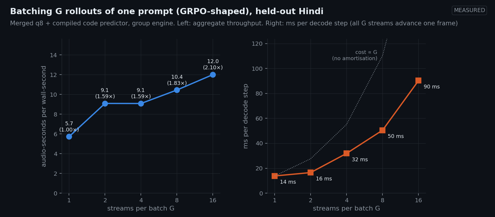
G	Throughput	vs. G = 1	Step	Batch latency	Peak memory
1	5.72 audio-s/s	1.00×	13.8 ms	1.27 s	6.5 GB
2	9.08	1.59×	16.5 ms	1.56 s	8.2 GB
4	9.08	1.59×	31.9 ms	3.25 s	8.3 GB
8	10.44	1.83×	50.5 ms	5.63 s	9.7 GB
16	12.00	2.10×	90.3 ms	9.68 s	9.9 GB

Rows running past their own EOS while waiting for the slowest one aren’t the cause — 90–95% of computed frames are useful. Why longer sentences batch worse than short ones is not explained yet, and it matters, because G = 4 is my GRPO group size (§9). Mean CER stayed in 0.08–0.10 across G, but on 40 clips per G, unpaired, that is a description, not a quality result.

One hypothesis tested and ruled out. A natural suspect for the jump between G = 2 and G = 4 is MLX switching quantized-matmul kernels (matrix-vector to matrix-matrix) at some batch size. bench_kernels.py --sections batch times every projection shape and the attention call at G = 1…16 in isolation. Per-call times grow smoothly — no step at 2 → 4. Summing those kernels over a frame (28 Talker and 75 code-predictor layer calls) predicts the measured step to within ~20% at G = 1 and 2, but not beyond:

G	Kernel sum (matmul + attention)	Measured step	Unexplained
1	11.9 ms	13.8 ms	1.9 ms
2	13.6 ms	16.5 ms	2.9 ms
4	18.4 ms	31.9 ms	13.5 ms
8	26.4 ms	50.5 ms	24.1 ms
16	41.4 ms	90.3 ms	48.9 ms

So the stall is outside the matmul and attention kernels: something whose cost grows with G — per-row sampling and penalty, per-row bookkeeping, or the non-matmul ops at batch. The isolated kernels are a lower bound (no norms, RoPE or sampling; attention approximated at 100 and 400 cached keys), but the gap opens too abruptly to be those alone. Not yet located.

One more finding: my GRPO trainer’s rollout sampler (sample_rollouts_interleaved) already batched the group — I had assumed it didn’t. Wiring the compiled code-predictor frame into it (opt-in fast_code_pred) is bit-identical on the four tensors Phase B replays and 1.24× faster on a small check (3 prompts × 2 seeds, G = 4, LoRA unmerged as in training) — a correctness check with a timing attached, not a training-speed result.

What changes at scale

On a server the shape of the problem changes. vLLM-Omni runs Qwen3-TTS as two stages — the Talker (stage 0) and Code2Wav (stage 1) — each with its own batching and its own decoder chunking. On two H20s in voice-clone mode, mean time-to-first-packet was 70.61 ms at c = 1 and 1,127.93 ms at c = 64; their stacked Qwen3-TTS optimizations took c = 64 throughput from 26.55 to 42.88 audio-seconds per second (+61.5%). The paper’s own table gives the 12 Hz 0.6B model 97 ms to first packet and RTF 0.288 at concurrency 1.

One loop vs. two stages. At serving scale the Talker and the decoder become separate stages with their own batches and chunk sizes, so neither waits on the other. Schematic.

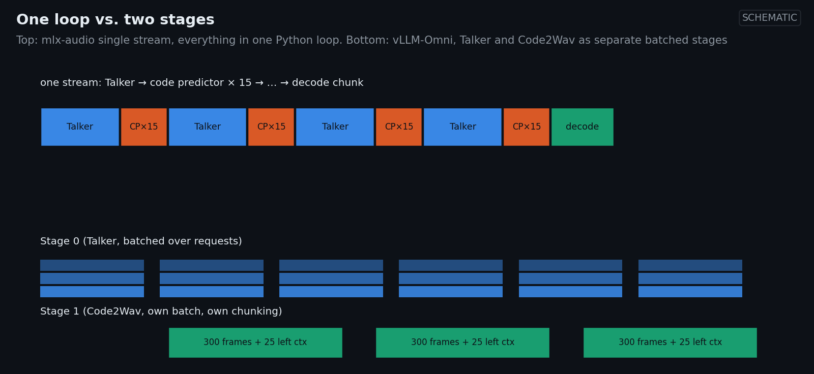
None of those numbers is comparable to a laptop. What transfers is the structure: separate the decoder from the token loop, batch each on its own terms, and chunk the decoder independently of what you ship.

---

9. What’s still open

What this run establishes

Stated as narrowly as the evidence allows: on an M5 Pro, merging the Hindi GRPO LoRA into the 8-bit base and compiling the code predictor’s fifteen passes make Qwen3-TTS 0.6B 1.56× faster single-stream (3.19× → 4.98× real-time, drift-corrected), with no statistically significant degradation in Whisper CER or DNSMOS — and intervals inside stated margins — on 300 unseen sentences. After those changes the largest 8-bit matvecs, in isolation, move weights at about the DRAM spec, and the frame sits ~1.5× off the first-order roofline. It does not establish that the output sounds the same to Hindi listeners, and it says nothing about batching beyond a preliminary sweep.

Open items

• Blind listening by native Hindi speakers. Every quality result in this post is automatic: Whisper CER and an English-trained DNSMOS. The accepted ladder has never been blind-rated. What I’d count as evidence: several native speakers, randomised A/B pairs from held-out sentences, a “same” option, and a pre-stated threshold for what preference rate is a regression — with attention to retroflex and aspirated consonants and to pacing, which §5.8 showed a change can move without touching CER. The A/B page generator is in the harness (scripts/make_ab_listening.py).
• The fused-kernel ceiling: ~1.2×. 30% of a compiled code-predictor frame is not matmul work; at ~1.9 µs per kernel and many hundreds of kernels per frame, a fused code-predictor layer via mx.fast.metal_kernel could recover part of it. Metal has no public device-wide barrier, so each layer still needs about four kernels (one per matmul). CUDA experience (fused elementwise kernels: 1.1–1.25× end to end) suggests the realistic gain is at the lower end.
• Why batching stalls past G = 2. In the preliminary sweep, G = 4 stalls at 1.59× on realistic utterances, against 2.2× on short ones. A kernel-path switch is ruled out (§8); 13.5 ms per step at G = 4 sits outside the matmul and attention kernels and hasn’t been located. The sweep itself needs more sentences, repeats and drift correction before it’s a number.
• Streaming. All time-to-first-packet numbers use mlx-audio’s default 2 s first chunk (25 frames). The paper’s 4-frame (320 ms) packets, and decoding with left context independent of the shipped chunk size, were not swept.
• Overlapping the decoder with generation (decode chunk N while generating chunk N+1): ~1.8 ms per frame is on the table.
• The model is the next lever. With the matmuls at the hardware, the structural cost is fifteen sequential code-predictor passes reading 72% of the bytes. Predicting several codebooks per pass, or distilling a smaller code predictor, could be worth more than everything above — but that is training, not inference.
• The training side. LoRA dropout during RL and evaluation, the repetition penalty mismatch between GRPO sampling and deployment, and SFT not beating the base model on an unseen corpus are all questions for the next training post.

Closing

The two changes that worked were not clever. One removed work the deployed model had been doing by accident — an adapter that was never merged. The other removed launches from the one component that was launch-bound, which the roofline had pointed at before any code was written. Everything else either hit the hardware or failed the quality gate, and the measurement problems were harder than the optimisations.

That is the systems lesson I’d carry forward: predict first, profile the profiler, change one thing at a time, and don’t trust a number until you know what else the machine was doing.

---

Appendix: reproduce it

Everything above was produced by a small harness in mlx-audio-train, built on top of stock mlx-audio 0.4.4. Every lever is one switch; every run writes one ledger row plus its evidence. The file map and commands are folded away below.

Files and commands (click to expand)

File	What it does
bench/levers.py	The lever registry: every change in §5, by name
bench/fast_generate.py	A copy of mlx-audio’s decode loop with the loop levers: device-side penalty, async eval, compiled code-predictor frame, compiled Talker step, fast sampler; plus the batched group engine (§8)
bench/lora_merge.py	Merging QLoRA into the base (bf16 or requantized q8)
bench/quantize.py	Requantization, whole-module or selective (MLP only)
bench/fuse_proj.py	Fused QKV and gate/up projections
bench/decoder_compile.py	Bucketed compiled codec decoder
bench/quality.py	The quality gate: CER/DNSMOS scoring, bit-exactness, sentence-level bootstrap CIs and non-inferiority margins, noise-aware speed check
bench/telemetry.py, bench/env.py	macmon GPU telemetry, contention detection, environment snapshot
scripts/bench_tts.py	One configuration → one ledger row (speed, TTFP, component split, quality, gate)
scripts/bench_sweep.py + bench/sweeps/	Run a YAML list of configurations, each in a fresh process, resumable
scripts/bench_profile.py	The level-by-level profiler with sync-cost calibration (§4)
scripts/bench_kernels.py	Per-kernel cost, matvec efficiency, frame decomposition (§4); matmul and attention cost vs. batch size (§8)
scripts/bench_batch.py	The batch-size sweep (§8)
scripts/bench_teacher_forced.py	Teacher-forced code-predictor comparison: record a reference’s frames, replay them through variants, compare distributions (§5.8)
scripts/make_prompt_set.py, scripts/make_ab_listening.py	The held-out prompt set; the blind A/B listening page

The runs behind this post:

# held-out set (100 IndicTTS-Hindi sentences)
python scripts/make_prompt_set.py --n 100 --seed 0 --out bench/prompts/hi_indictts_100.jsonl

# the ladder: baselines + every lever, 300 clips each, one ledger row per configuration
export BENCH_LEDGER=path/to/qwen3tts_mlx_ledger.csv
python scripts/bench_sweep.py bench/sweeps/m5pro_part4.yaml --keep-going
python scripts/bench_sweep.py bench/sweeps/m5pro_part4_extra.yaml --keep-going

# one configuration by hand: GRPO adapter + the two accepted levers
python scripts/bench_tts.py --config configs/qwen3_tts_hindi_grpo.yaml \
    --adapter <grpo adapters.safetensors> --variant hindi-grpo \
    --levers lora-merge-q8,compile-code-pred --lever compile-code-pred \
    --config-id my-run --prompts bench/prompts/hi_indictts_100.jsonl

# profiler, kernel microbenchmark, batch sweep
python scripts/bench_profile.py --config configs/qwen3_tts_hindi_grpo.yaml --adapter <...> --tag grpo-q8 \
    --prompts bench/prompts/hi_smoke.txt --level all
python scripts/bench_kernels.py --adapter <...>
python scripts/bench_kernels.py --sections batch

# quality confirmation on 300 new sentences (rows 100-400 of the same shuffle), and
# the teacher-forced code-predictor check
python scripts/make_prompt_set.py --n 400 --seed 0 --out bench_runs/hi_indictts_400.jsonl
#   (then take rows 100-400 as bench/prompts/hi_indictts_confirm300.jsonl)
python scripts/bench_tts.py ... --prompts bench/prompts/hi_indictts_confirm300.jsonl --num-prompts 300 --seeds 0
python scripts/bench_teacher_forced.py --adapter <...> --n 20 --variants unmerged,cp-q4,cp-q4-g32,cp-mlp-q4
python scripts/bench_batch.py --config configs/qwen3_tts_hindi_grpo.yaml --adapter <...> \
    --levers lora-merge-q8 --engine group --groups 1,2,4,8,16 --seeds 0,1 \
    --prompts bench/prompts/hi_indictts_100.jsonl --num-prompts 20 --variant hindi-grpo --config-id batch

python scripts/bench_tts.py --list-levers prints every lever and whether it is expected to be bit-exact. The GRPO trainer change from §8 is opt-in: fast_code_pred: true under grpo: in the config.

---

References

Qwen3-TTS and its implementations

• Qwen3-TTS Technical Report — Qwen Team, 2026
• Qwen3-TTS-12Hz-0.6B-Base config
• mlx-community/Qwen3-TTS-12Hz-0.6B-Base-8bit
• mlx-audio — Prince Canuma and contributors
• MLX — Apple
• mlx-audio-train (harness in bench/) — akashicMarga
• qwen3-tts-hindi-lora — akashicMarga
• IndicTTS-Hindi — SPRINGLab

Optimization work on Qwen3-TTS and similar models

• faster-qwen3-tts — andimarafioti
• qwen3-tts-triton
• I Made a Single CUDA Kernel Speak — Jayanth Kumar Morem
• Qwen3-TTS on Apple Silicon — Soniqo
• FluidAudio and mobius — FluidInference
• Engineering TTS Inference in vLLM-Omni — vLLM-Omni TTS Team, 2026
• fast-dacvae — kadirnar
• VoiceHub TTS model benchmarks — kadirnar

Inference engines and tools

• ML Drift: Scaling On-Device GPU Inference for Large Generative Models — Tang et al., 2025
• Decode performance optimizations for MLX inference (issue #3789)
• macmon — sudo-free Apple Silicon monitor

This series

• Running Conversational AI Locally (roofline method)
• prefill-decode-bench
• From Spectrograms to Speech Codecs
• Inside the Speech LM
• GRPO Post-Training for TTS

---

Animations generated with Manim Community. Render scripts: qwen3tts_mlx_bytes_per_frame.py and qwen3tts_mlx_sync_lanes.py in /assets/animations/. Charts generated from _data/qwen3tts_mlx_ledger.csv and _data/qwen3tts_mlx_abba.json by /assets/charts/qwen3tts_mlx_figures.py. Benchmark harness, profiler and evidence: bench/ and scripts/bench_*.py in mlx-audio-train.

---

<

Previous Post

Teaching a Speech Model to Judge Itself: GRPO Post-Training for TTS on Apple Silicon

>

Blog Archive

Archive of all previous blog posts